

CodeWalkthrough: Image Stitching with OpenCV
A pit-stop on my journey to Structure-from-Motion

Image stitching is a pit-stop on my journey to learn how to do 3D reconstruction from 2D images, also known as Structure-from-Motion (SfM). I’m hoping this would familiarise myself to the common concepts and libraries before I attempt SfM which would undoubtedly be harder.
Image stitching or photo stitching is the process of combining multiple photographic images with overlapping fields of view to produce a segmented panorama or high-resolution image.
In this post, I’ll be going through my attempt at image stitching using Python and OpenCV. I also used the University of Maryland CMSC246 Computer Vision course and various tutorials (most notably here and here) to guide my learning.
Since my aim is to learn the concepts, I did not use ready-made functions in OpenCV for this work. Neither did I go crazy and started to code everything using Numpy. Instead, I tried to strike a middle ground by using helper functions in OpenCV that would calculate key quantities like key features and homography matrices that would be used to build towards a stitched image.
As usual, I encourage the reader to look through the code repo to follow along. For the impatient reader, the key Jupyter notebook that we’ll be looking through is here.
Image stitching process
The image stitching process involves at least 2 images. For every pair of images, I1 and I2, the following steps are performed to create a single image.
Feature Detection
The first step is to detect notable features in both images. A feature in an image are things like corners and edges. The usefulness of the image feature would also depend on its surrounding pixels. Like the red dots shown in the picture below.
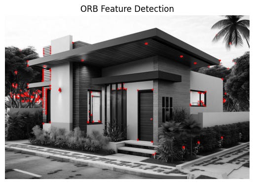
These are points which would be informative when determining whether an object exists in pictures taken from different perspectives.
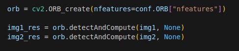
In this work, I used the ORB feature detector in the match_features function. The ORB feature detector calculates the coordinates of the key features as well as descriptors for each feature. Descriptors are arrays of numbers that encode key characteristics of the feature, much like embeddings in the LLM-space.
Feature Matching
The next step is to match the features in both images to each other. That is to say for example, the corner of the table in picture 1 is the same as that in picture 2.
Take the picture of Lenna below. On the left, I have a cropped and rotated image. On the right I have the full image. The red dots are the features detected individually in the previous step. The green lines are the features that are matched to each other. As can be seen, the eyes are matched to each other and there’s a single point on the nose that is matched in both images.
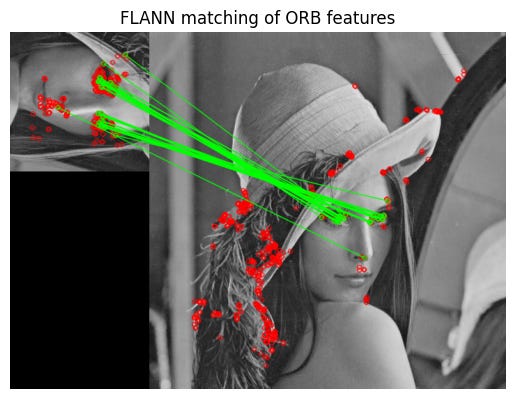
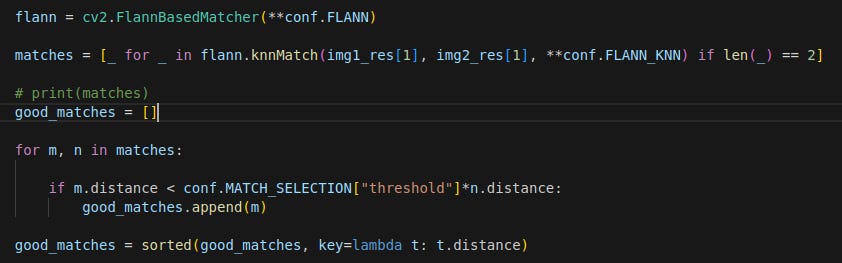
I used the FLANN feature matcher in this work. There is also a small filtering step to filter away weak matches.
Homography Matrix Calculation
Now we reach the crucial step, figuring how to transform one image to match the other by calculating the homography matrix, which describes how an image transforms from one camera’s perspective to another.
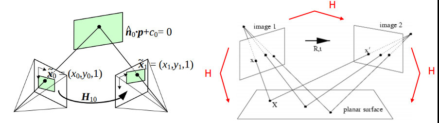
Seen below, the homography matrix H describes how a feature coordinate in I1, (x, y), transforms to the coordinates in the I2, (x’, y’).
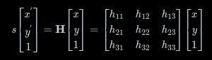
Using the findHomography function in OpenCV, we find a homography matrix that best transforms all the matched features in I2 to the same coordinates in I1.
Say we have both images shown below, with the features matched. The mountain images are taken from the CMSC246 course.
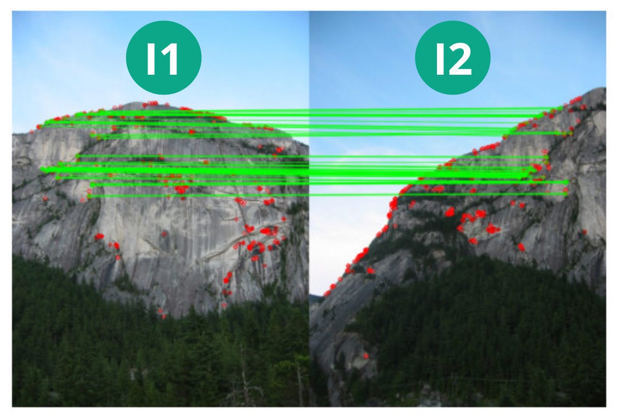
The homography matrix will help transform I2 to I1 as shown below. The steps to do so are in the next section.
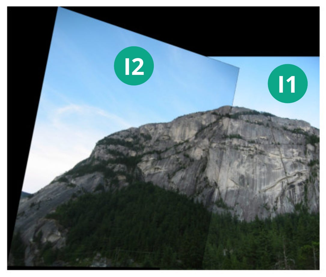
Something to note here is that the matched key features should be well distributed across the entire image in order for the homography matrix to be well calculated. If the matched key features are concentrated in a small area in the image, then only the area where the features are found will be well transformed and the rest of the image might not.
Image Merge
Final step. Merge I1 and I2 into one image.
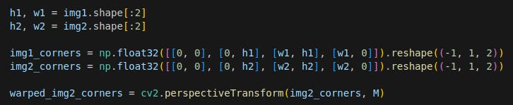
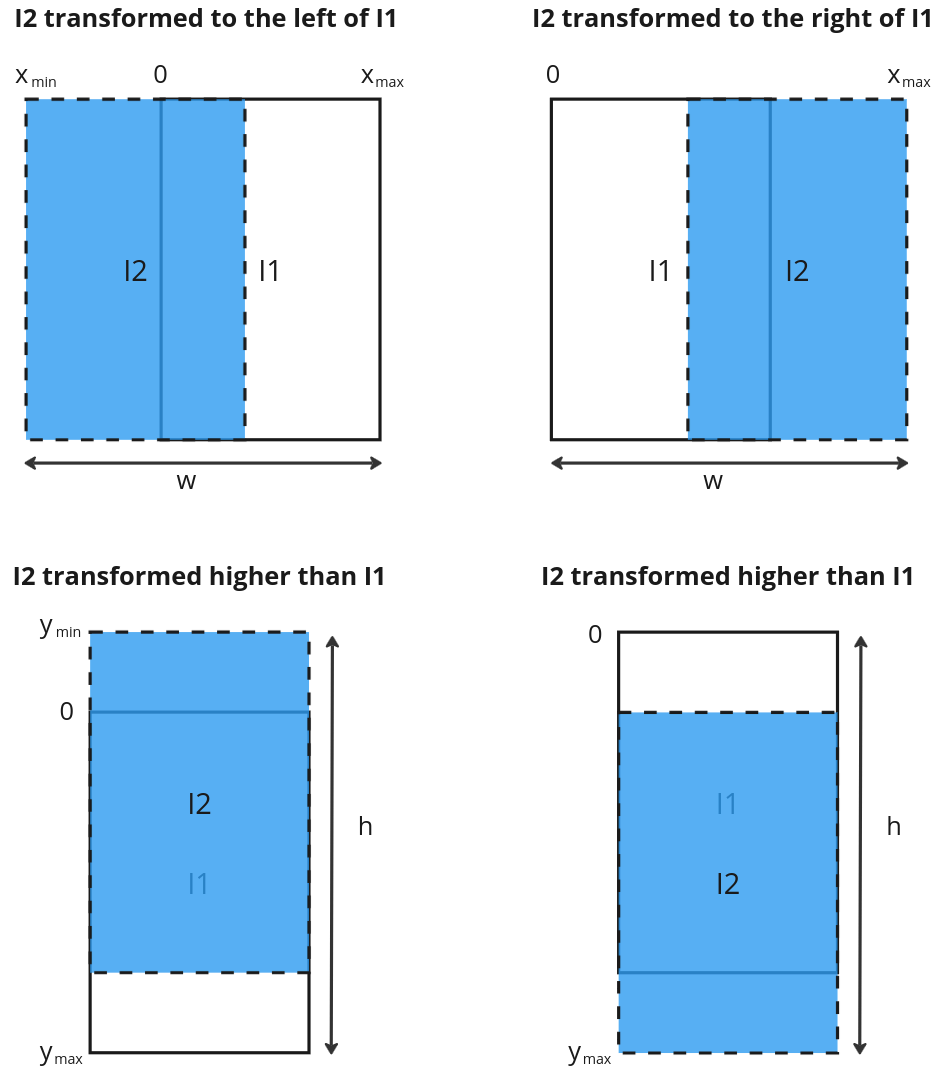
First, transform the corners of I2 using the homography matrix with the perspectiveTransform function. This would help figure out the final dimensions the merged image. As can be seen in the example above, the final image will be bigger than the individual images and I2 can end up higher/lower or to the left/right of I1, depending on the matched features. By transforming the corners of I2, the corners will end up with a coordinate relative to I1. See merge_images function.
We then figure out the size of the final image.
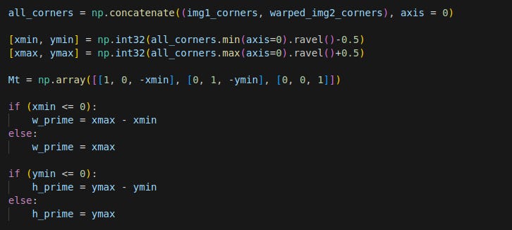
The logic to get the final width, w and height, h, is shown below.
I2 is then transformed using the warpPerspective function, where M is the homography matrix.

Note here that there is another matrix Mt that is multiplied to M. This is a translation homography matrix that shifts I2 without rotation to account for the fact that the top left corner of I2 is no longer (0, 0). To see the effect of Mt, look at this notebook.
The 2 images are then added together using a mask matrix.

Overall algorithm
The overall process to merge a set of images is as follows:
Given a set of images, set one image as I1 and another as I2.
Merge I1 and I2 using the above process to result in I3.
Set I3 as I1.
Select another image as I2 and repeat steps 1 to 3 till all the images are merged
Final output
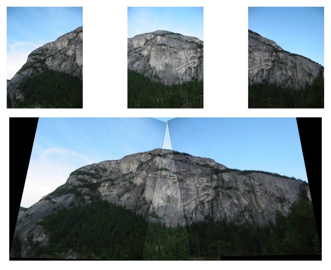
I made two examples. One of a mountain panorama (taken from the CMSC246 course).
And another one of a picture of Mount Fuji by Danill K from Unsplash.
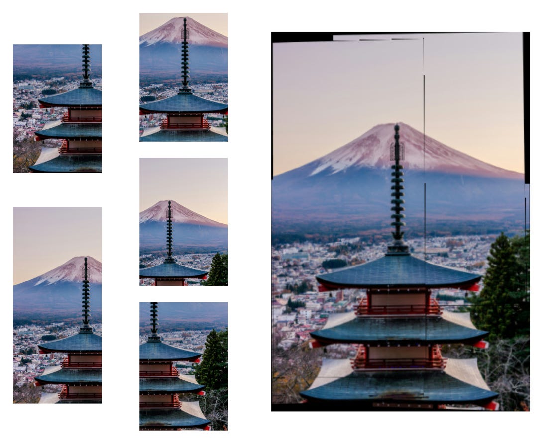
Final remarks
I was stumped for a while first by the step involving the calculation of the final dimensions of the merged image and the need to include Mt in the homography matrix before transforming I2. Took a while to visualise the operations and figure out why all my images were turning out gibberish.
The final outputs were also not perfect. You can see the edges of the constituents images and some edges are not as well aligned. The exposure across images is also not consistent. However to get all the details perfect would take a lot more. See the example of the openCV pipeline here.
OpenCV provides a convenient class that can perform image stitching easily. The output can be seen below. The output is much better.
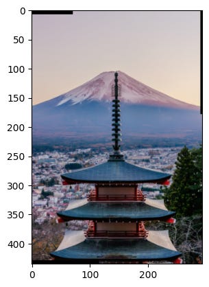
Nonetheless, this exercise has taught me about the key concepts behind image stitching. That’s enough for now.
Time to move on to structure-from-motion!