MathWalkthrough: Bellman's Principle of Optimality

If you know how to make good decisions, you need only to consider your next step.

Introduction

The Bellman’s Principle of Optimality is an important idea in the study of sequential decision making processes. It has found its way into many areas from software algorithms to inventory management in the form of dynamic programming and reinforcement learning.

In this post, I would like to describe the general idea behind the Bellman’s Principle of Optimality. I won’t go deeply into specific application of the principle but really try to take a look at its mathematical form and see what it means. I believe it will be easier to apply the principle once we can appreciate the general idea.

Problem Setup

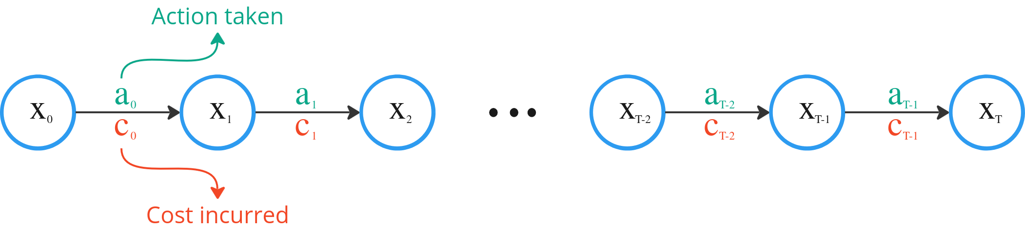
Consider a decision problem over T time steps. At any given time t, our environment is described by a state x_t. This “state” is simply the collection of “things” that tells us about the environment we are in. It could be temperature in the case of an oven. Or it could be the position, velocity and acceleration in the case of a car.

At each time step t, we have to make a decision d_t given the state x_t that would lead to an action a_t.

\(a_t = d_t(x_t)\)

We can think of d_t like a decision rule that tells us what to do when given situation described by x_t. For example, when the traffic light turns red, hit the brakes.

And as a consequence of a_t, our environment changes from x_t to x_t+1. Mathematically we can describe such a change using a transition function, Φ, which describes how the state changes given an action.

\(x_{t+1} = \Phi(x_t, a_t)\)

With our action, there also comes a cost, c_t(x_t, a_t).

As an example, when we step on the brakes while driving (action), the car slows down (state change) and we use more fuel during our journey (cost).

The overall process is shown below.

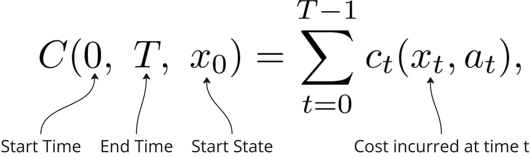
Thus we can express the total cost of all our actions over T time steps as a sum of all the costs incurred at each time step, C, as follows,

Taking a closer look at the total cost expression, we can write it in two ways. First, in the forward time direction, where it is the sum of the cost at time 0 plus the total cost from t=1 to t=T. This is how we experience things, starting at the start time and progressing forwards.

The second way is backwards in time, where we have the total cost up to the second last time step plus the cost at the last time. This is more like the planning way of thinking where we start with the end in mind and work our way back.

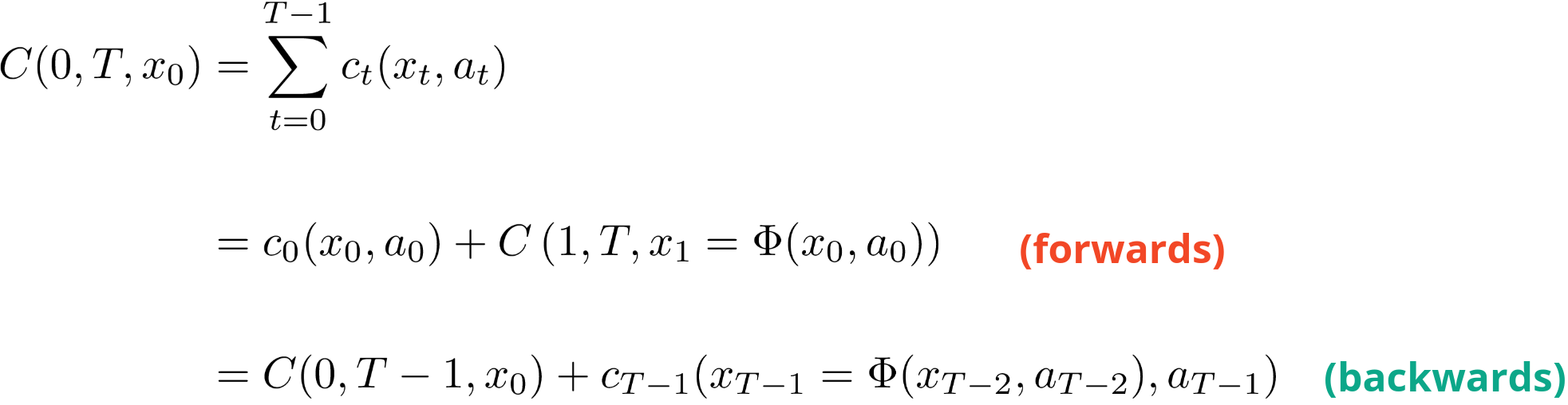
In both cases, notice the term where the next state is dependent on the previous state. This introduces the dependency of the costs incurred from the actions taken over the course of the time horizon.

For example, taking a closer look at the second term for the forward direction, the cost from t=1 to t=T is a result of x₁ which in turn is the result of the action taken at t=0, a₀ at state x₀.

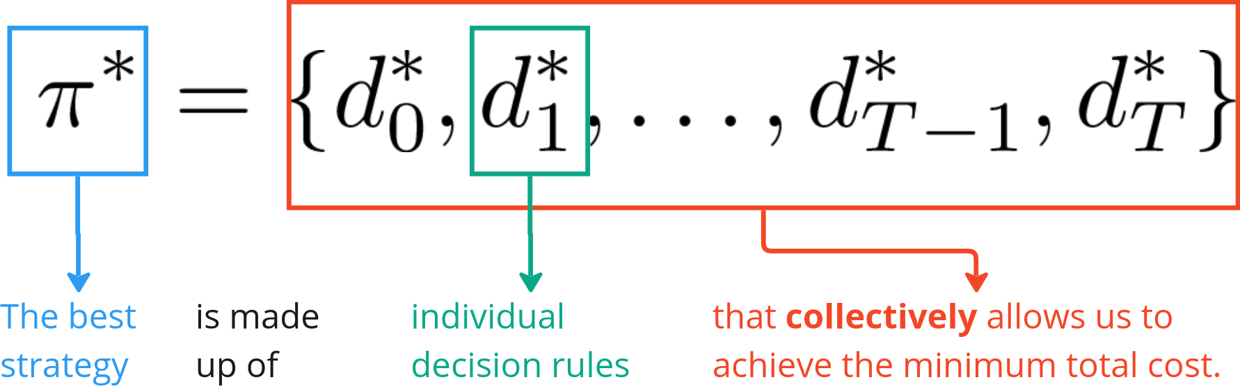
Lastly, to introduce one last piece of math machinery, the collection of all the decision rules is called the policy, π.

\(\pi = \{d_0, d_1, \ldots, d_T\}\)

Some call it a strategy. It is a way of thinking that informs us what decisions to take at each point in time under any given situation.

Now we are ready to start looking at the Bellman’s Principle of Optimality.

Bellman’s Principle of Optimality

Let me first quote the Bellman’s Principle of Optimality so that we can come back to it later.

Principle of Optimality: An optimal policy has the property that whatever the initial state and initial decision are, the remaining decisions must constitute an optimal policy with regard to the state resulting from the first decision. [Bellman1957]

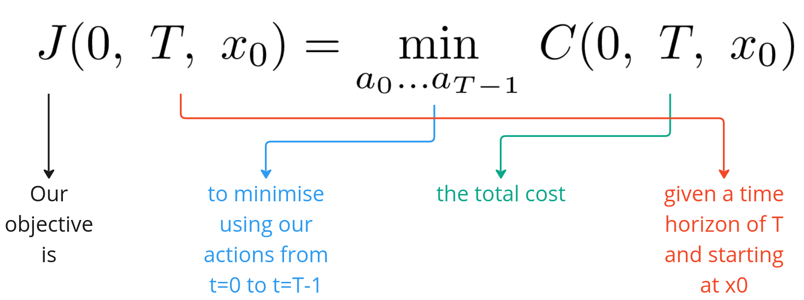
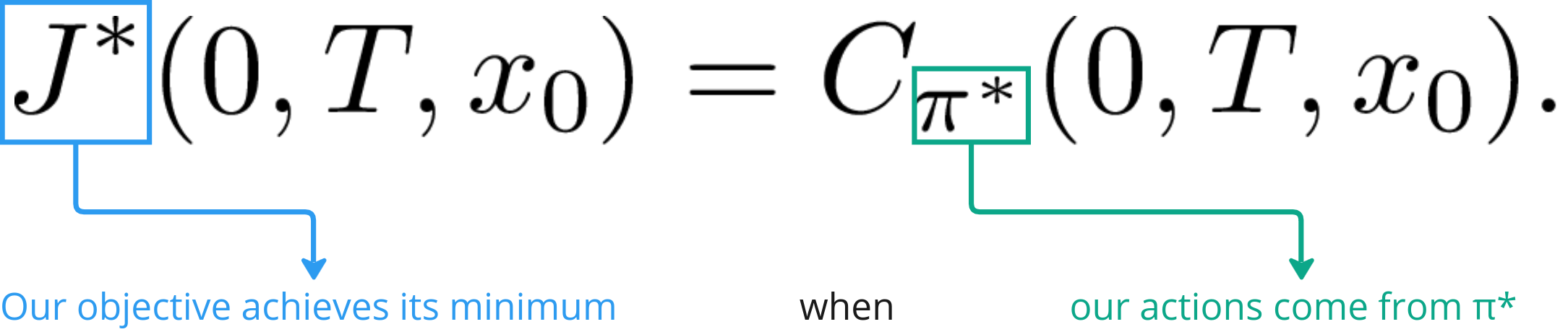
Our overall objective is to minimise the total cost over our time horizon T and is expressed below

Now suppose we are able to arrive at an optimal policy, π*, which gives us the best decisions rules that we can have such that the total cost is at its minimum. In other words,

Expanding the total cost expression, we have

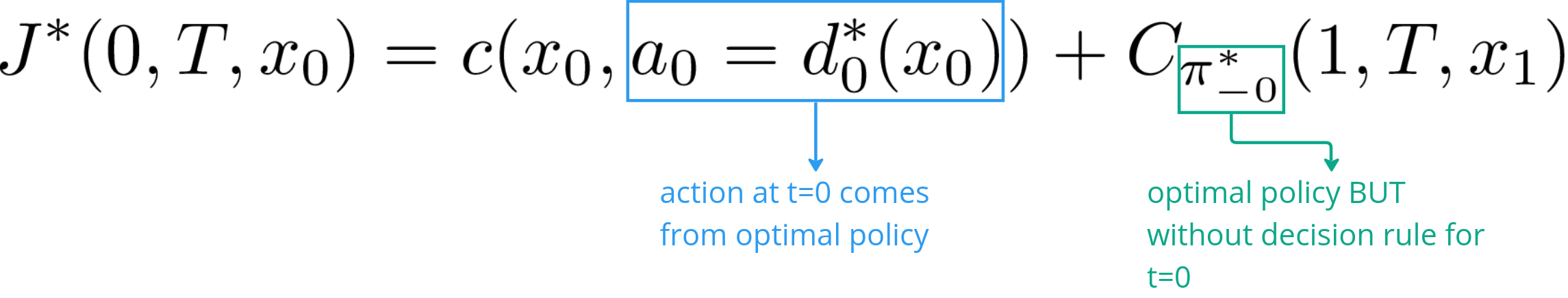
The above expression means that at t=0, we take an action that is optimal and leads us to state x₁ (first term) and follow the optimal policy thereafter (second term), we will arrive at a total cost that is the smallest it can be.

Now consider if we didn’t take the first action, a₀ according to the optimal policy, we would have

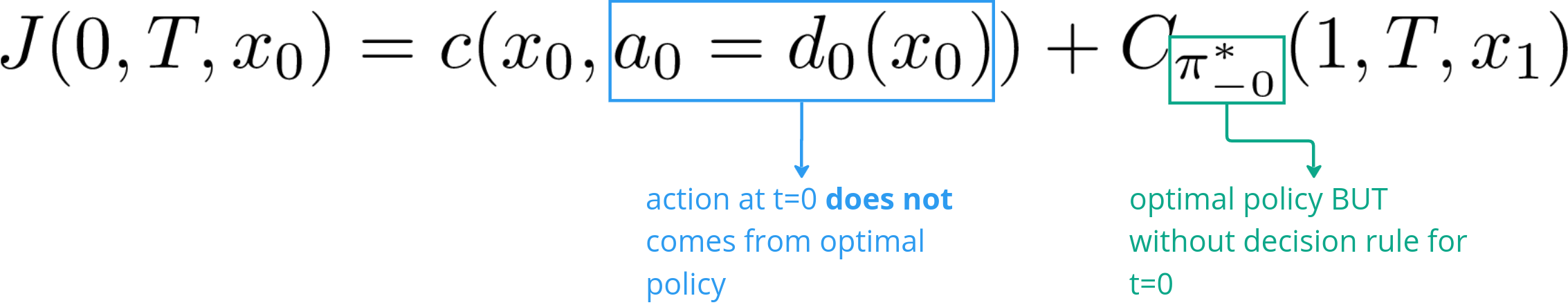
Of course, the total cost in this case would be greater or equal to the case where all actions were taken according to the optimal policy. But Bellman’s Principle of Optimality states that, by following the optimal policy after t=0, we would still arrive at the minimum cost given the initial state and action.

Two things to note here. Firstly, a policy is not a sequence of states. We do not specify the best path for the system to traverse through. Instead it is a sequence of decision rules (using our current nomenclature). That is why even if we didn’t make the optimal decision at t=0, our remaining policy decision rules will still be able to guide us to the best possible outcome given that we made a “mistake” initially by not following the optimal policy. Again, this does not mean that there is no cost to our mistake. The actual outcome would likely be worse than the optimal one just that it is the best that could have been achieved given the circumstances.

Secondly, the Bellman’s Principle of Optimality highlights the importance of knowing how to make good decisions and if we know how to make good decisions, then we only need to worry about the next step. This is because make the first good decision would set us on the path to get to a good state where we can make the next good decision to get us to the next good state and so on and so on.

The keen-eyed reader would notice at this point that while the Principle of Optimality is all well and good, it is not clear as to how one would arrive at an optimal policy. For that, I can only refer the reader to full length treatments by Sutton [Sutton2018] and Bertsekas [Bertsekas2020].

Problem Variations and Additional Considerations

In this article, I have used a simplified context to present the Principle of Optimality. There are variations and additional considerations that makes the Principle widely applicable in many situations. Here are some of them.

Rewards instead of Costs

In some cases, rewards are considered instead of costs. This is a simple modification to our treatment of the Principle here. Rewards are simply negative costs or vice versa. So in dealing with rewards we maximise instead of minimise. In books where rewards are used, you would see the total cost function being called the value function. See [Sutton2018].

Continuous Actions

If instead of discrete actions like start or stop, you have actions that can take continuous values such as how much to steer, then you would also approximate the decision rules as functions. In fact, you can approximate the entire policy as a policy function. See [Sutton2018].

Continuous Time

We have dealt with discrete time steps in this article. The time steps could be 1 second each, or 1 hour, 1 day, 1 month, doesn’t matter. But the shorter the time interval represented by each step the closer we come to considering things in continuous time where we would have to use the mathematical apparatus of stochastic differential equations (SDEs). Interested readers might consider look at [Hassler2015] and [Oksendal2014].

Stochasticity

In this article, I have assumed that the transition from one state to another is deterministic. In other words, if a particular action is taken at a particular state, it will always lead to a known next state. This is not true in general. There is unpredictability present and the next state will be one of many possible states each with its own probability of occurrence.

To that end, the objective function stated above will have to be augmented with an expectatoin over all possible states. In other words, we will have to weight the costs of each possible next state according to their likelihood of occurrence.

This means that the optimal policy would give you the best outcome on average. But not that on any particular “run” or “episode” you are not guaranteed to always achieve the lowest cost or highest rewards.

I won’t dwell too much on this. Interested readers can refer to [Sutton2018] and [Bertsekas2020].

Books by R. Howard [Howard2007a, Howard2007b] also offer very good insights on how to treat non-deterministic state transitions in Markovian systems.

Conclusion

Bellman’s Principle of Optimality is an interesting concept that I picked up when I was into reinforcement learning and dynamical systems. I have found it applicable not just in the technical arena but also in life when thinking about decision making.

References

[Sutton2018] R.Sutton, A. Barto, 2018, Reinforcement Learning: An Introduction

[Bertsekas2020] D. Bersekas, 2020, Dynamic Programming and Optimal Control: Volume 1, 4th edition

[Bellman1957] R. Bellman, 1957, Dynamic Programming

[Hassler2015] U. Hassler 2015, Stochastic Processes and Calculus: An elementary introduction with applications

[Oksendal2014] B. Oksendal, 2014, Stochastic Differential Equations

[Howard2007a] R. Howard, 2007, Dynamic Probabilistic Systems: Markov Models (Volume 1)

[Howard2007b] R. Howard, 2007, Dynamic Probabilistic Systems: Semi-Markov and Decision Processes (Volume 2)