TurboQuant for Document Retrieval

A step-by-step walkthrough of the TurboQuant algorithm

Imagine a chat between a user and a Large Language Model (LLM). It is a to and fro of queries and responses between the LLM and the user. Each time the user responds, the entire chat is sent to the LLM so that the response can be computed. The thing is, the only thing that changes to the chat each time is the latest response from the user. Most of the earlier messages remain the same. A key-value cache allows an LLM to reuse previously computed values from earlier messages to predict the next token quickly instead of recalculating all the required values again. One can imagine how useful and cost saving this can be when serving LLMs at scale.

As the context windows of LLMs (i.e. the total length of a chat an LLM can sustain) gets longer, the key-value cache also gets larger. To the point where the cost of holding all this in high-speed memory is becoming quite significant, especially at scale. Key-value caches are usually held in high-speed in-memory stores that are not cheap.

TurboQuant is a compression algorithm by Google that address the problem of high memory consumption by key-value caches as the context length of LLMs grow. It also has the effect of making similarity searches more effective thereby making applications like vector retrieval (think Retrieval Augmented Generation) more efficient.

In this post, I describe my efforts in building TurboQuant from scratch and walk you through the details of the algorithm, the way I understand it. As with walkthrough posts on thoughtsre, it would be most effective if the reader follows along with the code in this GitHub repository. I will also be posting links to the exact code locations in the repository as we go along.

Why I am interested in TurboQuant

To be honest, I got interested in TurboQuant not really because it can help serve LLMs prediction quickly. My curiosity was piqued when the authors mentioned that the algorithm is data oblivious.

For example, in order for Retrieval Augmented Generation (RAG) to work well, not only do the documents to be searched need to be chunked and embedded (i.e. converted into an array of numbers so that the LLM can “intuit” about its contents), the “patterns” across the documents also need to be discovered so that the vector database used to store the document can easily find the relevant documents, potentially amongst millions. What this means is that some form of clustering algorithm needs to be run on the documents so that when matching a query to a potential document, only the most similar clusters need to be searched. Importantly, this clustering needs to be run periodically as new documents are added.

TurboQuant negates that need. It doesn’t need to know what documents are already in and what documents might come. This is also why this walkthrough is about document retrieval. It’s what got me interested and also serves the purpose of helping me understand how TurboQuant works (and also I’m GPU-poor).

Beyond that, I’ve always felt that AI models (not necessarily transformer-based) will one day communicate with each other via some neuralese language and it would have to be data oblivious and highly compressed. TurboQuant might hold some insights into that. Another reason why I was motivated to build it myself.

Experiment Methodology

I used the Kaggle arXiv dataset as the raw material for the document retrieval process. The sentence transformer miniLM model was used to create the initial embeddings, with a length of 384, for the documents which are then treated with the TurboQuant algorithm. A user query can then be treated using the TurboQuant algorithm again and matched to the closest article in the document cache.

The embeddings were generated by concatenating the title and the abstract. Articles with abstracts shorter than 150 characters were removed.

In this experiment, I’ve also used Polars as my main processing engine, simply because I’ve always wanted to learn it be could never find the chance to do so.

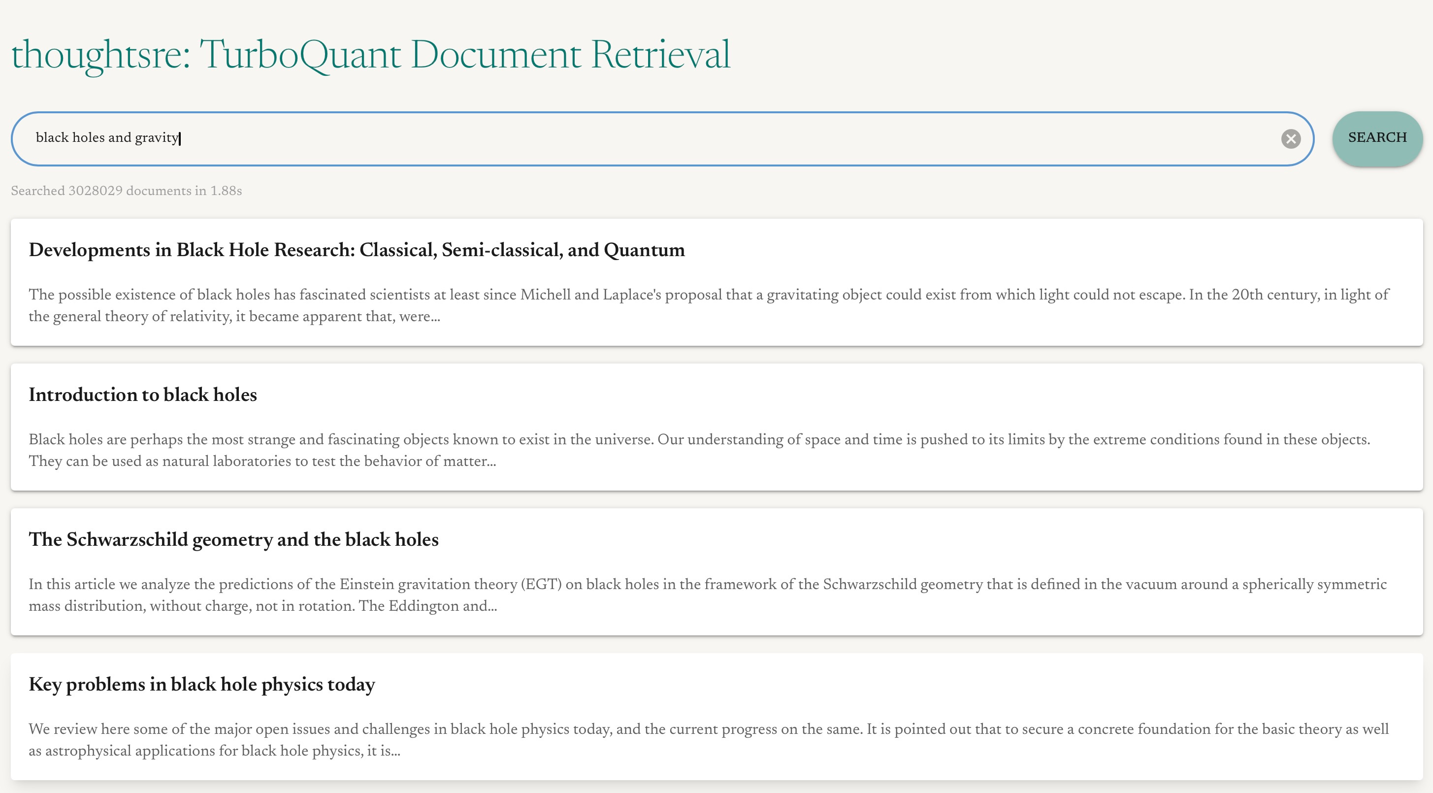
The interested user can run the demo in the GitHub repository to try it out. A screenshot is shown below. The demo searches through 3 million documents in ~1.5-2s. This is highly un-optimized. My purpose is to understand the algorithm.

TurboQuant overview

I won’t go through the math or the proofs on performance bounds. The reader can read the paper for that. In a nutshell, the algorithm works by quantising the raw embeddings which exists as floats into a binary representation (we’ll get into that later). Even without getting into too much detail we can already see how it can lead to a reduction in memory usage. If a single float that takes 32 bits (float32) can be compressed to represent roughly the same amount of information while using only 4 bits, that’s an 8 times reduction in memory cost! The difference between TurboQuant and other existing quantisation techniques is that the steps it takes allows it to not care about how each value in the embedding vector is distributed in relation to each other and instead is only dependent on the coordinate itself. This allows it to derive its computational benefits.

The algorithm consists of 2 main parts. The first part, let’s call it MSE, seeks to minimise the reconstruction error after quantisation and results in a representation of b bits per embedding coordinate. The second part, let’s call it QJL (after the Quantised Johnson-Lindenstrauss algorithm), is used to correct for biases in MSE part. In the context of document retrieval, both parts are used to calculate some similarity to a user query of each document to retrieve the one with the most relevant content, although using the MSE part alone might work well enough for document retrieval already.

By the way, an embedding coordinate refers to a particular value in the embedding vector. So if an embedding vector has a length of 384, it is a 384 dimension vector and the i-th element is the i-th coordinate.

Step-by-step walkthrough

On the whole, TurboQuant algorithm’s encoding process goes like this (Parts 2 and 3 of the encoding process are repeated for each document in the dataset. The overall code to create all TurboQuant embeddings is here.):

Encode - Part 1: Setup (DONE ONCE ONLY)

Decide how many bits should be used to represent each embedding coordinate.

The more bits the more accurate the reconstruction of the embeddings will be but the lower the compression. I chose a 4-bit representation which would quantise each coordinate into 2^4=16 clusters. More explanation on what that means in the next step.

Calculate the codebook which gives the centroids to quantise each embedding coordinate.

The centroids or clusters each embedding value is assigned to are given by the Max-Lloyd algorithm on a Beta distribution (more on why a Beta distribution and why this is important later). Computationally, this means you run K-means on a bunch of samples from a Beta distribution and each centroid is a K-means cluster. The number of centroids will depend on the number of bits used. The more bits, the more cut points, hence the greater reconstruction accuracy. For example, 4 bits means you run a 16 cluster K-means clustering.

What this does is that, given a 4 bit representation for each coordinate whose value follows a particular Beta distribution, it creates a fixed set of values (or centroids) which divides the distribution into 16 sections where each section roughly has the same amount of “mass” or in this case “probability”.

This is calculated once for every single coordinate. We’ll see why later.

Select random seeds for embedding rotation

In the paper, the authors use the random rotations quite a bit to “mix” up the coordinates of the embeddings. However, if your embedding is 384-dimensional, that means the rotation matrix is a 384x384 matrix. And having to do the matrix multiplications for such a high-dimensional vector and matrix is computationally expensive.

Enter the Fast Walsh-Hadamard Transform (FWHT). When applied 2-3 times consecutively, it converges towards the same effect as a random rotation matrix. A closer look at the algorithm will remind the reader that it’s like shuffling cards. To get a good random shuffle, you do it a few times. Although, in the code shown, I only rotated the embeddings once as it was good enough for my purposes.

A thing to note about FWHT is that it acts on vectors with dimensions that are a power of 2. This is because it basically repeatedly segments the vector into 2 equal halves and calculates the sum and differences between the halves. In the code, if the input vector has length of 384, you will end up with a rotated vector of 512.

So what basically happens is that instead of storing the entire 384x384 matrix and having to do full matrix multiplication each time, we replace the rotation with FWHT which is a fast algorithm. However the important thing to note here is the FWHT requires the generation of random sign flips and that the rotation has to be consistently performed across all documents and queries in order for FWHT to simulate the effect of a single random rotation matrix rotating all embeddings. Otherwise, we’ll just be performing random rotation of embeddings, randomly.

So we select 2 random seeds for our rotation. One for the MSE stage and one for the QJL stage. In the code I chose the seed for MSE and QJL to be 42 and 24, respectively.

Encode - Part 2: MSE stage

In this stage, we put a lot of the things we created during the Part 1 setup stage to use. I will explain the how and why as we go along.

Rotate each embedding using a random rotation.

The embedding can be a key/value embedding (if used in LLMs) or a document embedding (if used in RAG). This random rotation via FWHT will result in a vector where each coordinate is independent of each other in the limit of high-dimensions and will follow a Beta distribution that is symmetric around 0 for its values.

This is why TurboQuant is data oblivious. It doesn’t matter what the overall distribution of values across all the embedding coordinates is. This rotation step will always guarantee that the resultant coordinate-wise distribution of values goes to a Beta distribution (or even a Normal distribution at high dimensions).

The random sign flips required by FWHT also got me thinking about how models can be personalised or data access can be controlled. Say if a set of documents were rotated using a particular random number generator seed and another set of documents were rotated using the same algorithm but a different seed, technically speaking these two sets of documents would not be compatible with each other! This is because they would be rotated into different “spaces”. The random seed then sort of becomes some from of encryption key, if you will. In the case of FWHT being applied repeatedly, then it is the sequence of random seeds used to generate the random flips which is the “key”.

Another important note is that all the embeddings should be a unit vector.

Quantise the embedding by representing each coordinate according to the index position of the codebook centroid to which the coordinate value is closest to.

This in a way is like assigning a sample point to a particular K-means cluster. In this way, each coordinate, ordinarily represented by a float, can now be represented via an integer. The value can be recovered with the help of the codebook. For example, if a particular coordinate has a value of “2” at the end of this step, it means that the value is closes to the centroid in the codebook at position “2”. This step is done here in the code and the logic is here.

So at the end, given N samples of 512 dimensional (each of which are floating point numbers) embeddings, you will end up with N samples of 384 assignments of coordinates to centroids where each of the 512 assignments are integers (in our case uint8). From a memory usage point of view, going from a float32 representation to a uint8 representation is already a 4x compression, even without changes in overall matrix dimensionality.

Pack the bits for further compression.

If say 4 bits were used in this stage, then you can further pack the bits in adjacent embedding coordinates so that 2 embedding coordinates can be represented using a single 8-bit integer. Why is this so? Remember that each embedding coordinate is now represented by a number between 0 (inclusive) and 16 (i.e. 0, 1, 2, 3, …, 15) for the 4 bit representation which we have chose. There are no other numbers since we only have 16 centroids. This means that although each embedding coordinate uses a uint8 which takes up 8 bits, only the right-most 4 bits out of the 8 is ever used.

This means that we can actually combine the 2 numbers (each using only 4 bits) into 1 number (using all 8 bits fully). Specifically in our case, the length 512 uint8 vector can be packed into a length 256 uint8 vector.

So what we do is, as shown in diagram below,

• For each pair of embedding coordinate, bit-shift the first one to the left by 4 bits

• Perform and OR operation

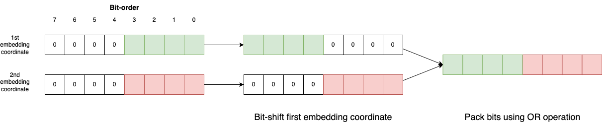
So now, instead of 2 uint8 numbers, we only need one. Another 2x compression. The core logic is here.

Encode - Part 3: QJL stage

The entire QJL encoding stage is in this code block.

Calculate the residuals from the reconstruction of MSE into the original embedding.

This involves taking the quantised embedding and 1) recovering the actual centroid values associated with each coordinate, 2) reversing the rotation and 3) calculating the coordinate-wise difference between the reconstruction and the original to get the residual vector. This step is performed here.

The residual vector in this case is a 384-dimensional vector corresponding to the original embedding dimensions.

The interesting thing here is that the inverse FWHT operation is simply FWHT itself using the same seed! See here. Again, no complicated calculations of inverse matrices and high-dimensional matrix multiplications. Simply apply FWHT again.

Rotate the residuals and take the sign of each of the residual coordinate-wise.

This is actually the QJL algorithm where this stage gets its name from. The result is a single binary for each coordinate. In the code itself, instead of storing +/-1, the result is stored as a boolean, where “0” means less than or equal to zero and “1” otherwise.

This time you rotate the residuals using the random seed selected in Part 1 specifically for the QJL step. This is a separate rotation. That’s why it is important to use a different seed to seed the sign flips.

Again, using FWHT, gives us a 512-dimensional rotated residuals vector.

Pack the bits for further compression.

There is no need to store the signs of each residual coordinate as an integer or a boolean, since each value can be represented as a single bit. Eight of them, for example, can be packed into a single 8-bit integer. This results in a 64-dimension vector (512/8).

Calculate the norm of the residual vector

The norm of the residual vector is then calculated. This is to correct for the bias-ness of the MSE stage reconstruction (See Section 3.2 of the paper).

A note on data sizes

To illustrate the differences in data sizes, the raw 384 dimensional embeddings stored in float32 is 6.71GB. The bit-packed quantised embeddings without the QJL stage is 792MB. The bit-packed quantised embeddings with the QJL stage is 1GB because other than the QJL bits, we also store the residual norm.

Encoding user queries and matching documents

As mentioned before, TurboQuant is data oblivious and its centroids are constant. This gives it an advantage over traditional RAG in document retrieval in the sense that it does not have to learn the document space via techniques like K-means (I’m sure there are more sophisticated methods) to find centroids which can be used to reduce the search space. This is a good point to mention that the TurboQuant “centroids” are not the same as the K-means “centroids” in conventional RAG.

The K-means “centroids” are points in the embedding space that are cluster centers. In other words, if the embedding is 384-dimensional, then the centroid is also a 384-dimension vector. TurboQuant “centroids” are per embedding coordinate. This is also because the coordinate values are almost independent at high-dimensions after rotation, as mentioned in the paper.

The document retrieval process goes like this (the reader can see the whole process in the query method of the TurboQuant client):

Encode the user query into an embedding vector.

This is done using the Sentence Transformer embedding language model, resulting in a 384-dimension vector.

Rotate the query embedding and quantise the embedding using the codebook centroids.

Same as Encode - Part 2: MSE stage, rotate the query using FWHT with the random seed used for the MSE stage. This transforms the embeddings into the same space as the document embeddings prior to quantisation and bit-packing. There is no need to bit-pack the rotated query embeddings this is because we will be doing things in a faster way in the next step.

Create a lookup table for all the quantised values to the cosine similarity from the centroids to calculate the MSE distance.

Algorithmically, this step is interesting. We could have followed the encoding steps to quantise and bit-pack the query embedding so that we can send it to our document embedding database to be compared. But that would require unpacking the bits and then performing element-wise operations. That is highly inefficient.

TurboQuant has already given us all the information we need. After all, the centroids are constant and we already know the centroid assignments of each coordinate of the embeddings of each document. All we need now is a lookup table.

Using a lookup table is faster than unpacking the bits and calculating the distances one-by-one for each document. It reduces the mathematical operations into a lookup operation which is much faster.

Remember in the MSE stage, the centroid assignments for 2 consecutive coordinates are bit-packed into a single number. So for a 4-bit representation, there are 16 centroids per coordinate. Hence there are 16x16=256 possible pairs of centroid assignments. We can pre-calculate the product of the query embedding and the centroid value (not assignment) at each coordinate into a lookup table with 256 entries. We only need to do this once for each query across all document comparisons.

In this way, when we sum up the products of the query embedding and centroid value at each coordinate, we actually get the cosine similarity of the quantised document embedding with the query for the MSE stage.

Rotate the query using the QJL seed to calculate the QJL adjustment.

Using definition 1 in the paper, we then rotate the query, again with FWHT, using the QJL random seed. The dot product of the rotated query vector and the QJL bits (unpacked of course) are then multiplied by the residual norm (calculated in QJL stage) and a scaling factor (see here).

Sum both values to get the final similarity score of the query to the documents.

The highest score is the document that is most relevant to the query. See here.

And there you have it! A ranked selection of documents corresponding to a user query!

Final thoughts

First and foremost, it was really enjoyable to be writing code by hand and to feel that you own the codebase again. The only thing I vibe coded was the one-page demo UI. (I mean, if you’re not going to use AI to write throwaway demos then what are you going to use it for? Right?)

Secondly, TurboQuant represents a way to think about embeddings that I, personally, haven’t thought of before. The use of rotation to transform the space into a stable one that then has the effect of providing a lot of information up front (think about the lookup table step) that allows for efficient processing. This makes me think that there might be something there that allows for inter-model communication via neuralese language.

Third, the use a random rotation matrix (or of FWHT and the need for a stable seed) presents a way of preserving privacy in the sense that if the other party does not know what is the rotation matrix that should be used to decode the message, it will map the input embeddings to a different space which will result in gibberish outputs (I think).

Fourth, less of a thought and more of an admission of a cop-out. The paper uses the number of bits to mean both the MSE and QJL bits. In other words, the representation seen in this blog corresponds to a 5-bit TurboQuant according to the paper’s notation. This is something to note. I did this because if I had taken the paper’s notation, a 4 bit representation will end up with a 3-bit MSE representation and made the bit packing/unpacking together with the QJL bit excessively complicated for the purpose of this exercise. So what I did was I did the MSE stage in 4 bits and just store the QJL parts additionally.

Lastly, as mentioned at the beginning, the implementation is highly unoptimised and is more suited for instruction than production. Searching 3 million docs in 1.5s is not fast by today’s standards. I had used Polars data frames as my “database”. A dedicated vector database would probably be faster (although at the time of writing I don’t think any of them implemented the TurboQuant search algorithm. I could be wrong). The paper itself also mentioned that the use of implementations such as the AVX2 In-register Lookup Tables will dramatically improve performance.